
OpenZFS Distributed RAID (dRAID) - A Complete Guide
(This is a portion of my OpenZFS guide, available on my personal website here.)
dRAID, added to OpenZFS in v2.1.0 and TrueNAS in SCALE v23.10.0 (Cobia), is a variant of RAIDZ that distributes hot spare drive space throughout the vdev. While a traditional RAIDZ pool can make use of dedicated hot spares to fill in for any failed disks, dRAID allows administrators to shuffle the sectors of those hot spare disks into the rest of the vdev thereby enabling much faster recovery from failure.
After a RAIDZ pool experiences a drive failure, ZFS selects one of the pool’s assigned hot spares and begins the resilver process. The surviving disks in faulted vdev experience a very heavy, sustained read load and the target hot spare experiences a heavy write load. Meanwhile, the rest of the drives in the pool (the drives in the non-faulted vdevs) do not contribute to the resilver process. Because of this imbalanced load on the pool, RAIDZ pool resilvers can potentially take days (or even weeks) to complete.
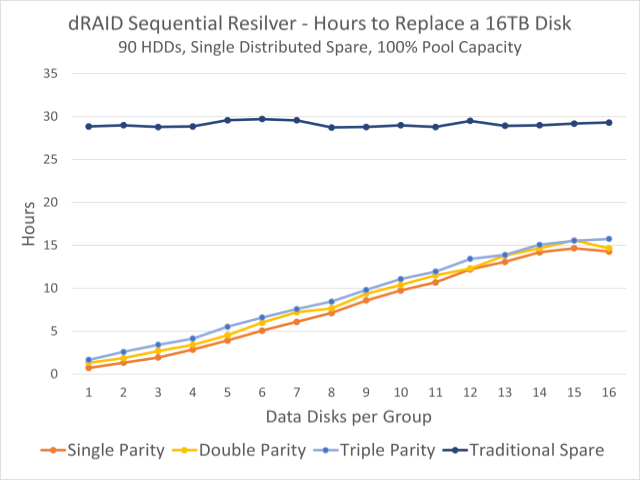
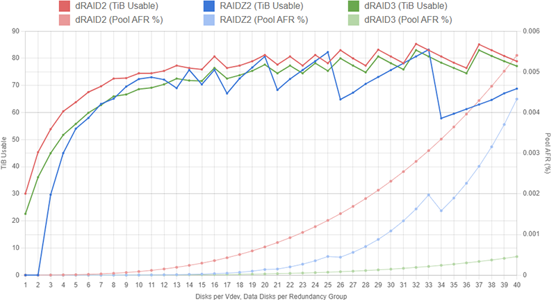
By contrast, after a dRAID pool experiences a drive failure, all of the disks in the faulted dRAID vdev contribute to the resilver process because all of the disks in the dRAID vdev contain hot spare space as well as data and parity information. With all of the drives more evenly sharing the recovery load, dRAID pools can resilver and return to full redundancy much faster than traditional RAIDZ pools. The chart below (from the official OpenZFS docs) shows the rebuild time of a traditional RAIDZ-based pool versus several dRAID configurations:
dRAID represents something of a paradigm shift for ZFS administrators familiar with RAIDZ. The distributed RAID technology introduces a number of new terms and concepts and can be confusing and intimidating for new users. We’ll outline everything you need to know in order to get started here and, for those interested, we will also dive into the weeds to see how this new vdev layout works.
dRAID Basics
If you create a new RAIDZ (Z1, Z2, or Z3) pool with multiple vdevs and attach a hot spare or two to that pool, ZFS effectively silos a given vdev’s data to the disks that comprise that vdev. For example, the set of disks that make up vdev #2 will hold some data and some parity protecting that data. Obviously, this vdev #2 will not have any parity data from any other vdevs in the pool. Hot spares also do their own thing: they don’t store anything useful and they just sit idle until they’re needed. Parity data within a given vdev is naturally distributed throughout that vdev’s disks by nature of the dynamic block size system RAIDZ employs; RAIDZ does not dedicate a particular disk (or set of disks) to hold parity data and does not neatly barber-pole the parity data across the disk like more traditional RAID systems do.
dRAID effectively combines all of the functions outlined above into a single, large vdev. (You can have multiple dRAID vdevs in a pool; we’ll discuss that below.) Within a dRAID vdev, you’ll likely find multiple sets of data sectors along with the parity sectors protecting that data. You’ll also find the spares themselves; in dRAID terminology, these hot spares that live “inside” the vdev are called virtual hot spares or distributed hot spares. A given set of user data and its accompanying parity information are referred to as a redundancy group. The redundancy group in dRAID is roughly equivalent to a RAIDZ vdev (there are important differences; we’ll cover them below) and we usually expect to see multiple redundancy groups inside a single dRAID vdev.
Because a single dRAID vdev can have multiple redundancy groups (again, think of a single pool with multiple RAIDZ vdevs), dRAID vdevs can be much wider than RAIDZ vdevs and still enjoy the same level of redundancy. The maximum number of disks you can have in a dRAID vdev is 255. This means that if you have a pool with more than 255 disks and you want to use dRAID, you’ll have multiple vdevs. There are valid reasons to deploy smaller vdevs even if you have more than 255 disks: you may want one dRAID vdev per 60-bay JBOD, for example. The number of disks in the dRAID vdev is referred to as the number of children.
Just like with RAIDZ, dRAID lets us choose if we want single, double, or triple parity protection on each of our redundancy groups. When creating a dRAID pool, administrators will also specify the number of data disks per redundancy group (which can technically be one but should really be at least one more than the parity level) and the number of virtual spares to mix into the vdev (you can add anywhere from zero to four spares per vdev).
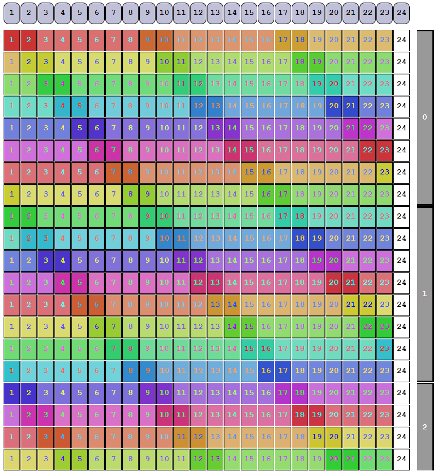
Somewhat confusingly, dRAID lets redundancy groups span rows. Consider a dRAID vdev with 24 disks, a parity level of 2, and 6 data disks per redundancy group. For now, we won’t use any spares so things line up nicely: on each row of 24 disks, we can fit exactly 3 redundancy groups:
(2 parity + 6 data) / 24 children = 3 redundancy groups
The layout (before it’s shuffled) is shown below:
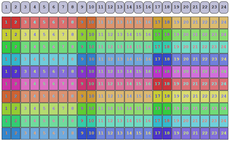
In this image, the darker boxes represent parity information and the paler boxes are user data. Each set of 8 similarly-colored boxes is a redundancy group. The purple boxes as the top of the diagram are labels showing the physical disks.
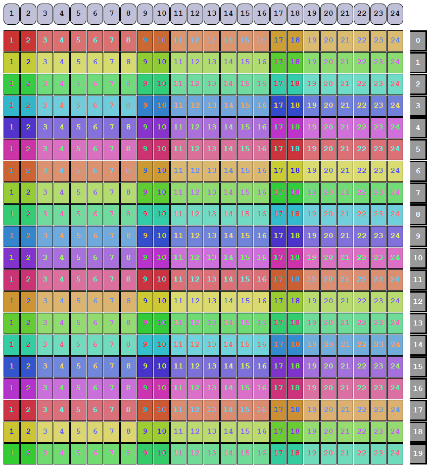
Although it’s counter-intuitive, we can actually add a spare to this dRAID vdev without increasing the number of child disks. The first row will have two full and one partial redundancy groups (as well as one spare): the third redundancy group will partially spill over into the second row. The layout (again, before it’s shuffled) is shown below:
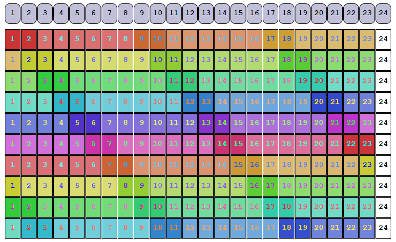
Because the virtual spare (represented here by the white blocks) does not need to be confined to a single physical disk, storage administrators have some additional freedom when designing dRAID layouts. This layout achieves the physical capacity of 17x disks almost as if we had 2x 6wZ2 vdevs, 1x 5wZ2 vdev, and a hot spare.
The dRAID notation is a bit cryptic, but once you understand the four variables at play, it starts to make sense. Again, the variables are the parity level (p), the number of data disks per redundancy group (d), the total number of child disks (c), and the total number of spares (s). The example above with 2 parity, 6 data, 24 children, and 1 spare would be annotated as:
draid2:6d:24c:1s
Because redundancy groups can span rows, the only real restriction here (other than those laid out above) is that the number of child disks must be at least as many as p+d+s. You can’t, for example, have the following layout:
draid2:21d:24c:2s
Obviously, we can’t fit 2 parity disks, 21 data disks, and 2 spare disks in 24 children and maintain double-parity protection on all the data.
dRAID Recovery Process
The primary objective of distributed RAID is to recover from a disk failure and return to full redundancy as quickly as possible. To that end, OpenZFS has created a new resilver process that is unique to dRAID called a sequential resilver.
Before diving into the sequential resilver, it will be helpful to review the traditional (or “healing”) resilver. When a disk fails in a pool with RAIDZ or mirrored vdevs, the subsequent resilver process will scan a massive on-disk data structure called the block tree. Scanning this block tree is not a simple, sequential process; instead, we have to follow a long, complex series of block pointers all over the pool. A block here may point to a block way over on the other side of the platter, which in turn points to some other blocks somewhere else. Walking through the entire block tree in this fashion takes a long time but it allows us to verify the integrity of every bit of data on the pool as we’re performing the operation; every block in ZFS contains a checksum of the blocks it points to further down the tree. Once the healing resilver has completed, we can be confident that our data is intact and corruption-free.
Obviously, the primary disadvantage of performing a full healing resilver is the extended time it can take to complete the procedure. During this time, our pool is highly vulnerable: subsequent disk failures could easily cause total data loss or, in the best case, drastically extend the period of pool vulnerability. dRAID aims to minimize that risk by minimizing the time that the pool is vulnerable to additional failures. This is where the sequential resilver comes in. As the name suggests, the sequential resilver simply scans all the allocated sections of all the disks in the vdev to perform the repair. Because the operations are not limited to block boundaries and because we’re not bouncing all over the disk following block pointers, we can use much larger I/O’s and complete the repair much faster. Of course, because we are not working our way through the block tree as in the healing resilver, we can not verify any block checksums during the sequential resilver.
Validating checksums is still a critical process of the recovery, so ZFS starts a scrub after the sequential resilver is complete. A scrub is basically the block-tree-walking, checksum-validating part of the healing resilver outlined above. As you might expect, a scrub of a dRAID pool can still take quite a long time to complete because it’s doing all those small, random reads across the full block tree, but we’re already back to full redundancy and can safely sustain additional disk failures as soon as the sequential resilver completes. It’s worth noting that any blocks read by ZFS that have not yet been checksum-validated by the scrub will still automatically be checksum-validated as part of ZFS’ normal read pipeline; we do not put ourselves at risk of serving corrupted data by delaying the checksum validation part of the resilver.
We’ve essentially broken the scrub into its two elements: the part that gets our disk redundancy back, and the part that takes a long time. A traditional resilver does both parts in parallel while the sequential scrub lets us do them in a sequence.
After the faulted disk is physically replaced, ZFS begins yet another new operation called a rebalancing. This process restores all the distributed spare space that was used up during the sequential resilver and validates checksums again. The rebalancing process is fundamentally just a normal, healing resilver, which we now have plenty of time to complete because the pool is no longer in a faulted state.
Other dRAID Considerations
As mentioned above, dRAID vdevs come with some important caveats that should be carefully considered before deploying it in a new pool. These caveats are discussed below:
-
Unlike RAIDZ, dRAID does not support partial-stripe writes. Small writes to a dRAID vdev will be padded out with zeros to span a redundancy group. This means that on a dRAID vdev with d=8 and 4KiB disk sectors, the minimum allocation size to that vdev is 32KiB. Essentially, this is the price that needs to be paid in order to support sequential resilvers. Given that, administrators should ensure they set recordsize and volblocksize values appropriately. If your workload includes lots of small-block data, running it on dRAID will likely create a lot of wasted space (unless you use special allocation classes; see below).
-
Because spare disks are distributed into the dRAID vdev, virtual spares can not be added after the vdev is created. This means that it is impossible to go from a
draid2:6d:24c:0sto adraid2:6d:24c:1swithout destroying the pool and recreating it. -
Performance of a dRAID vdev should roughly match that of an equivalent RAIDZ pool: vdev IOPS will scale based on the quantity of redundancy groups per row and throughput will scale based on the quantity of data disks per row.
-
Just as with RAIDZ, expansion of a dRAID pool requires the addition of one or more new vdev(s). Unlike RAIDZ, your dRAID vdev could have 100 or more disks in it. The ZFS best practice of using homogeneous vdevs in a pool still apply, meaning minimal expansion increments to a dRAID-based pool might be very large.
-
If you are creating a dRAID-based pool with more than 255 disks, you’ll need to use multiple vdevs. As above, adhering to best practices would mean keeping all vdevs alike, so rather than taking 300 disks and making one 255-wide vdev and one 45-wide vdev, consider either 2x 150-wide vdevs or 3x 100-wide vdevs.
-
Administrators can still attach L2ARCs, SLOGs, and special allocation class (“fusion”) vdevs to dRAID-based pools. Special allocation class vdevs were specifically designed to work with dRAID because they help to mitigate the poor efficiency and performance you might see when storing small blocks (particularly metadata blocks). Technically, you can also attach a normal hot spare to a dRAID pool but I honestly can not think of a reason why you would.
-
Leaving resilver time aside, a dRAID-based pool will almost always be more susceptible to total pool failure than a comparable RAIDZ pool at a given parity level. This is because dRAID-based pools will almost always have wider vdevs than RAIDZ pools but still have per-vdev fault tolerance. As discussed above, a pool with 25x 10-wide RAIDZ2 vdevs can theoretically tolerate up to 50x total drive failures while a dRAID configuration with 250x children, double parity protection, and 8 data disks per redundancy group can only tolerate 2x total disk failures. Once we consider the shorter resilver time of dRAID vdevs, the pool reliability comparison becomes a lot more interesting. This is discussed more below.
-
Although the concept of distributed RAID has existed in the enterprise storage industry for more than a decade, the ZFS implementation of dRAID is very new and has not been tested to the same extent that RAIDZ has. If your storage project has a very low risk tolerance, you may consider waiting for dRAID to be a bit more well-established.
When to use dRAID
Distributed RAID on ZFS is new enough that its suitable range of applications has not been fully explored. Given the caveats outlined above, there will be many situations where traditional RAIDZ vdevs make more sense than deploying dRAID. In general, I think dRAID will be in contention if you’re working with a large quantity of hard disks (say 30+) and you would otherwise deploy 10-12 wide Z2/Z3 vdevs for bulk storage applications. Performance-wise, it won’t be a good fit for any applications working primarily with small block I/O, so backing storage for VMware and databases should stay on mirrors or RAIDZ. If deployed on SSDs, dRAID may be a viable option for high-performance large-block workloads like video production and some HPC storage, but I would recommend thorough testing before putting such a configuration into production.
I’ve found the easiest way to approach the “when to dRAID?” question is to consider a given quantity of disks and to compare the capacity of those disks laid out in a few different RAIDZ and dRAID configurations. I built an application to graph characteristics of different RAID configurations to make this comparison process a bit easier; that tool is available here and will be referenced in the discussion below.
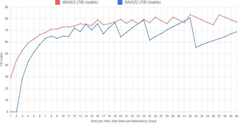
The graph below shows the capacity of several different RAIDZ2 and dRAID2 layouts with 100 1TB drives. The RAIDZ2 configurations include at least two hot spares and the dRAID2 configurations use two distributed spares and 100 children. The graphs show total pool capacity as we increase the width of the RAIDZ2 vdevs and increase the number of data disks in the dRAID layouts. We let both the RAIDZ2 vdev width and the quantity of dRAID data disks increase to 40.
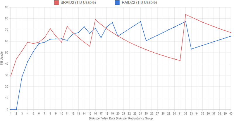
On both datasets, we see an interesting sawtooth pattern emerge. On the RAIDZ2 dataset, this is due to the vdev width getting close to being divisible by the total quantity of disks and then overshooting that and leaving lots of spare disks. When the vdev width is 24, we end up with four vdevs and four spare drives. Increasing the vdev width to 25 leaves us with three vdevs and 25 spare drives (remember, we’ve specified a minimum of two hot spares, so four 25-wide Z2 with zero spares would be invalid here).
The sawtooth pattern on the dRAID dataset is caused by partial stripe writes being padded out to fill a full redundancy group. Both datasets assume the pools are filled with 128KiB blocks and are using ashift=12 (i.e., drives with 4KiB sectors). A 128KiB block written to a dRAID configuration with 16 data disks will fill exactly two redundancy groups (128KiB / 4KiB = 32 sectors, which explains why we see another big peak at d=32). If we have 31 data disks in each redundancy group, a 128KiB block will entirely fill one redundancy group and just a tiny bit of a second group; that second group will need to be padded out which massively cuts into storage efficiency.
We can mitigate how dramatic this sawtooth shape is on the dRAID curve by increasing the recordsize. To make a fair comparison, we’ll increase the recordsize on both dRAID and RAIDZ2 to 1MiB:
Apparent usable capacity on both configurations has increased slightly with this change. The sawtooth pattern on the RAIDZ2 configuration set hasn’t gone away because we’ve only changed our recordsize, not how many disks fit into a vdev. The dRAID line is a bit smoother now because we’ve reduced how much capacity is wasted by padding out partially-filled redundancy groups. A 1MiB block will fill 256 data sectors (1024KiB / 4KiB = 256). If we have 31 data disks in each redundancy group, we end up with eight full redundancy groups and one partially-filled group that needs to be padded out. We’re still losing some usable space, but not nearly as much as before when the recordsize was 128KiB (one redundancy group with padding per eight groups full is much better than one group with padding for every one full).
We can clearly see that in most cases (especially the more “sane” cases where we limit the RAIDZ2 width to about 12 disks), dRAID eeks out a bit more capacity. As noted above, however, if we consider the pools’ resilience against failure, the dRAID2 configurations look less attractive:
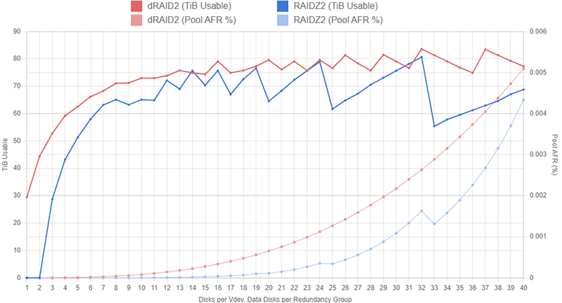
Because the dRAID vdev is so much wider and can still only tolerate up to two disk failures, it has a significantly higher chance of experiencing total failure when compared to the RAIDZ2 configurations. These annual failure rate (AFR) values assume the dRAID pool resilvers twice as fast as the RAIDZ pool for a given width.
By switching to dRAID3, we can actually drop the pool’s AFR by a considerable amount while still maintaining high usable capacity. For the following graphs, we’re going to limit the RAIDZ vdev width to 24 so it doesn’t throw off the AFR axis scale too much.
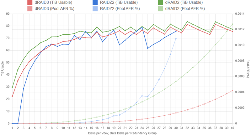
For reference, the dRAID2 configurations are shown here in green. The AFR of the dRAID configurations is considerably lower than the Z2 configurations across the board. As before, these AFR values assume the dRAID vdevs resilver twice as fast as the Z2 vdevs for a given width.
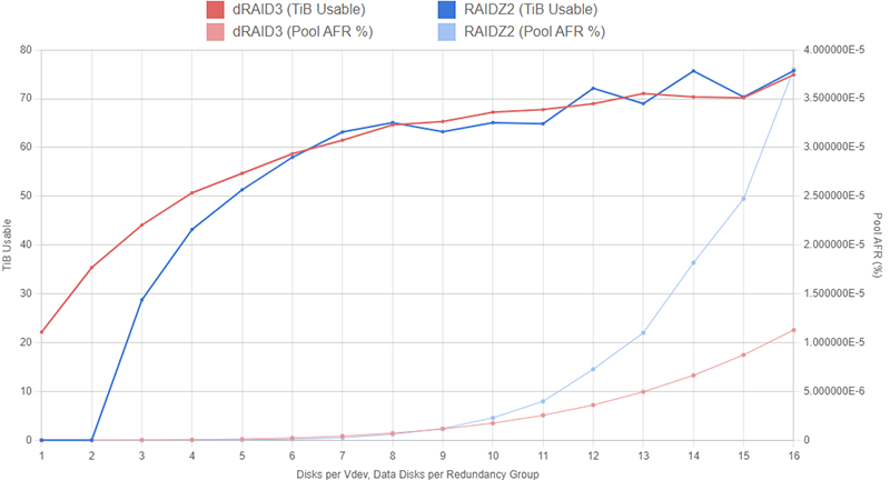
Even at d=16, the dRAID3 configuration has a roughly similar AFR to a 10-wide RAIDZ2 layout while offering more usable capacity. If you can stomach the lack of partial stripe write support and the large expansion increments, a dRAID3:16d:100c:2s pool may seem very appealing. Here’s a closer look at just the Z2 and dRAID3 configurations confined to 16 disks:
Before deploying this layout on brand new hardware, it should be noted that the pool AFR data on these graphs use a very simplistic model to predict resilver times and should not be taken as gospel. The model starts with an individual disk’s AFR, usually somewhere between 0.5% and 5%. We then try to estimate the resilver time of the pool by multiplying the vdev’s width (or the number of data drives in a dRAID config) by some scale factor. For the charts above, we assumed each data disk on a dRAID vdev would add 1.5 hours to the resilver time and each data disk on a RAIDZ vdev would add 3 hours to the resilver time (so a 12-wide RAIDZ2 vdev would take 30 hours to resilver and a dRAID vdev with d=12 would take 15 hours to resilver).
These 1.5 and 3 numbers are, at best, an educated guess based on observations and anecdotal reports. We can fiddle with these values a bit and the conclusions above will still hold, but if they deviate too much, things start to go off the rails. It’s also unlikely that the relationship between vdev width (or data drive quantity) and resilver time is perfectly linear, but I don’t have access to enough data to put together a better model.
You may also find that you can “split” the dRAID vdev in half to lower its apparent AFR. For example, if you compare 2x draid2:8d:50c:1s vdevs to 1x draid2:8d:100c:2s vdev, you’ll see the 2x 50c version has a lower apparent AFR across the board (keeping the resilver times the same). In reality, the 100c configuration should resilver much faster because it has 100 total drives doing the resilver instead of only 50; this will bring the AFR curve for the two configurations much close to each other. I don’t (yet) have data on how this scaling works exactly, but I’m curious to experiment with it a bit more.
If we had started out with 102 disks instead of an even 100, the RAIDZ2 configurations would have more capacity relative to the dRAID configurations because we can use (as an example) 10x 10wZ2 vdevs and still have our requisite two spares left. Here is a dRAID2, dRAID3, and RAIDZ2 configuration set with 102 drives instead of 100:
In cases where you have a nice round number of drives (like 60 or 100), dRAID may be preferable because it still lets you incorporate a spare without throwing the vdev width off too much. There is an option in the Y-Axis menu controls to show the number of spare drives for each layout; you’ll want to validate that your layout is not leaving you with a huge excess of spare drives.
I would encourage you to explore this graph tool a bit for yourself using parameters that match your own situation. Start by plotting out a few different dRAID and RAIDZ configurations, try changing the parity value a bit, check how changing the recordsize impacts the results too. Layer on the pool AFR curve and see how changing rebuild times impacts the results. If you find a dRAID topology that offers more capacity than a sensible RAIDZ topology, you might also check out the relative performance curves. Once you’ve absorbed as much data as you can, you’ll need to decide if that extra capacity is worth the dRAID tradeoffs and the little bit of uncertainty that comes with relying on relatively new technology.
dRAID Internals
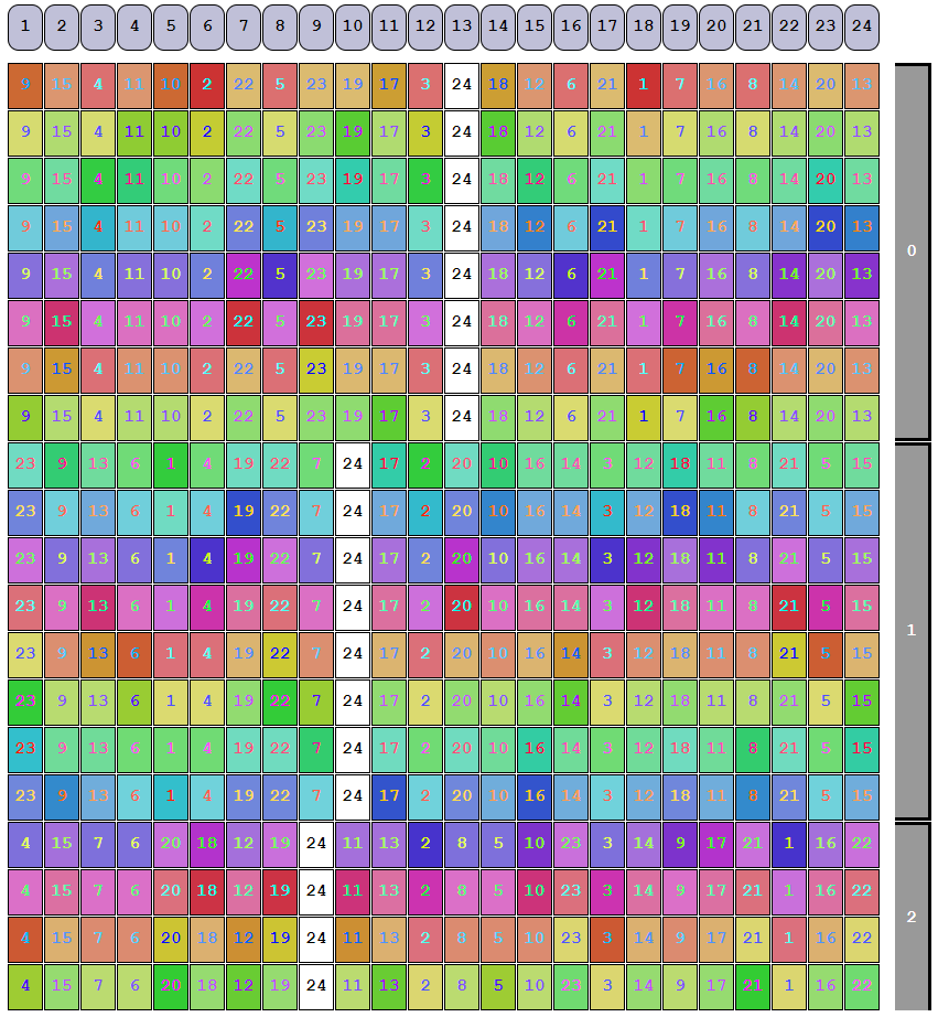
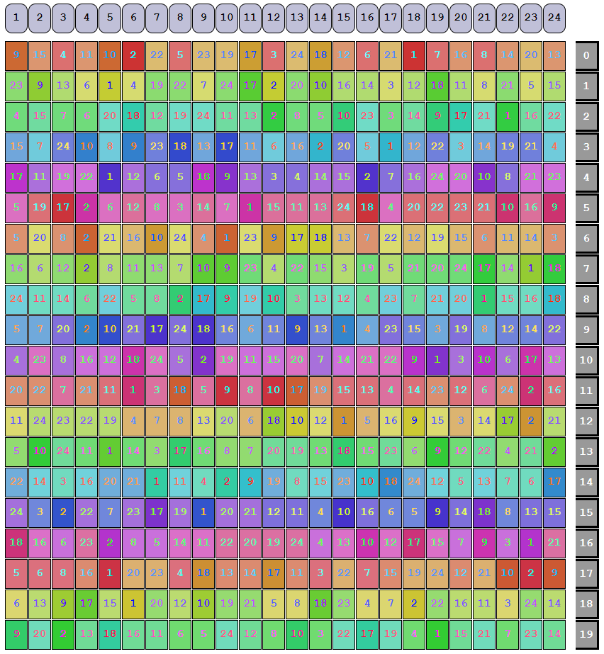
The layouts displayed with the examples above were not shuffled and thus do not represent what is written to the pool. When shuffling the on-pool data, ZFS uses hard-coded permutation maps to make sure a given configuration is shuffled the exact same way every time. If the permutation maps were ever allowed to change, un-shuffling terabytes of data would be an enormous task. The OpenZFS developers created a different permutation map for every value of c in a dRAID vdev (more specifically, they selected a unique seed for a random number generator which in turn feeds a shuffle algorithm that generates the maps).
Each row of the permutation map is applied to what dRAID calls a slice. A slice is made up of the minimum set of full rows we need to hold a full set of redundancy groups without any part of the last group spilling over into the next row. This is somewhat difficult to grasp without being able to visualize it, so the draid2:6d:24c:1s example from above is shown below with its slices noted:
Notice how 23 redundancy groups take up exactly 8 rows. If we work with any fewer than 8 rows, we’ll have at least one partial redundancy group. The number of redundancy groups in a slice can be determined by:
𝐿𝐶𝑀(𝑝+𝑑,𝑐−𝑠)(𝑝+𝑑)
The number of rows in a slice can be determined by:
𝐿𝐶𝑀(𝑝+𝑑,𝑐−𝑠)(𝑐−𝑠)
If the redundancy groups line up nicely (as they did in the draid2:6d:24c:0s example), then a slice will only contain a single row:
As we noted above, the permutation maps get applied per-slice rather than per-row. After shuffling, the draid6:2d:24c:1s vdev will be laid out as below:
Notice how within a slice, the rows in a given column all match; this is because all the rows in a slice get the same permutation applied to them.
Once shuffled, the draid6:2d:24c:0s vdev will be laid out as below:
As expected, each row gets a different permutation because our slice only consists of a single row.
When studying the above diagrams, you may intuitively assume that each box represents a 4KiB disk sector, but that is not actually the case. Each box always represents 16 MiB of total physical disk space. As the developers point out in their comments, 16 MiB is the minimum allowable size because it must be possible to store a full 16 MiB block in a redundancy group when there is only a single data column. This does not change dRAID’s minimum allocation size mentioned above, it just means that the minimum allocation will only fill a small portion of one of the boxes on the diagram. When ZFS allocates space from a dRAID vdev, it fills each redundancy group before moving on to the next.
The OpenZFS developers carefully selected the set of random number generator (RNG) seeds used to create the permutation mappings in order to provide an even shuffle and minimize a given vdev’s imbalance ratio. From the vdev_draid.c comments, the imbalance ratio is “the ratio of the amounts of I/O that will be sent to the least and most busy disks when resilvering.” An imbalance ratio of 2.0 would indicate that the most busy disk is twice as busy as the least busy disk. A ratio of 1.0 would mean all the disks are equally busy. The developers calculated and noted the average imbalance ratio for all single and double disk failure scenarios for every possible dRAID vdev size. Note that the average imbalance ratio is purely a function of the number of children in the dRAID vdev and does not factor in parity count, data disk count, or spare count. The average imbalance ratio for a 24-disk dRAID vdev was calculated at 1.168.
The developer comments note that…
…[i]n order to achieve a low imbalance ratio the number of permutations in the mapping must be significantly larger than the number of children. For dRAID the number of permutations has been limited to 512 to minimize the map size. This does result in a gradually increasing imbalance ratio as seen in the table below. Increasing the number of permutations for larger child counts would reduce the imbalance ratio. However, in practice when there are a large number of children each child is responsible for fewer total IOs so it’s less of a concern.
dRAID vdevs with 31 and fewer children will have permutation maps with 256 rows. dRAID vdevs with 32 to 255 children will have permutation maps with 512 rows. Once all the rows of the permutation maps have been applied (i.e., we’ve shuffled either 256 or 512 slices, depending on the vdev size), we loop back to the top of the map and start shuffling again.
The average imbalance ratio of a 255-wide dRAID vdev is 3.088. Somewhat interestingly, the average imbalance ratio of the slightly-smaller 254-wide dRAID vdev is 3.843. The average imbalance ratios show an unusual pattern where the ratio for vdevs with an even number of children is typically higher than those with an odd number of children.
The algorithm used to generate the permutation maps is the Fisher-Yates shuffle, the de facto standard of shuffle algorithms. The RNG algorithm used, called xoroshiro128++, is based on xorshift. In the dRAID code, this algorithm is seeded with two values to start the permutation map generation process: one seed that’s specific to the number of children in the vdev, and one hard-coded universal seed which, amusingly enough, is specified as 0xd7a1d533d (“dRAIDseed” in leet-speak when represented in hex).
dRAID Visualized
I’ve created an interactive dRAID vdev visualizer, available here. You can specify any valid dRAID layout and see it both in a pre-shuffled and a post-shuffled state. It uses the same RNG algorithm and seeds as the ZFS code, so it should accurately represent how everything gets distributed in a dRAID vdev. The average imbalance ratio of the vdev and the physical on-disk size of each box is displayed at the bottom.